Statistics
Counting Tanks and Taxis
How a serial number stamped on a gearbox let Allied statisticians out-estimate every spy in Europe, and why the arithmetic behind it fits on one line.
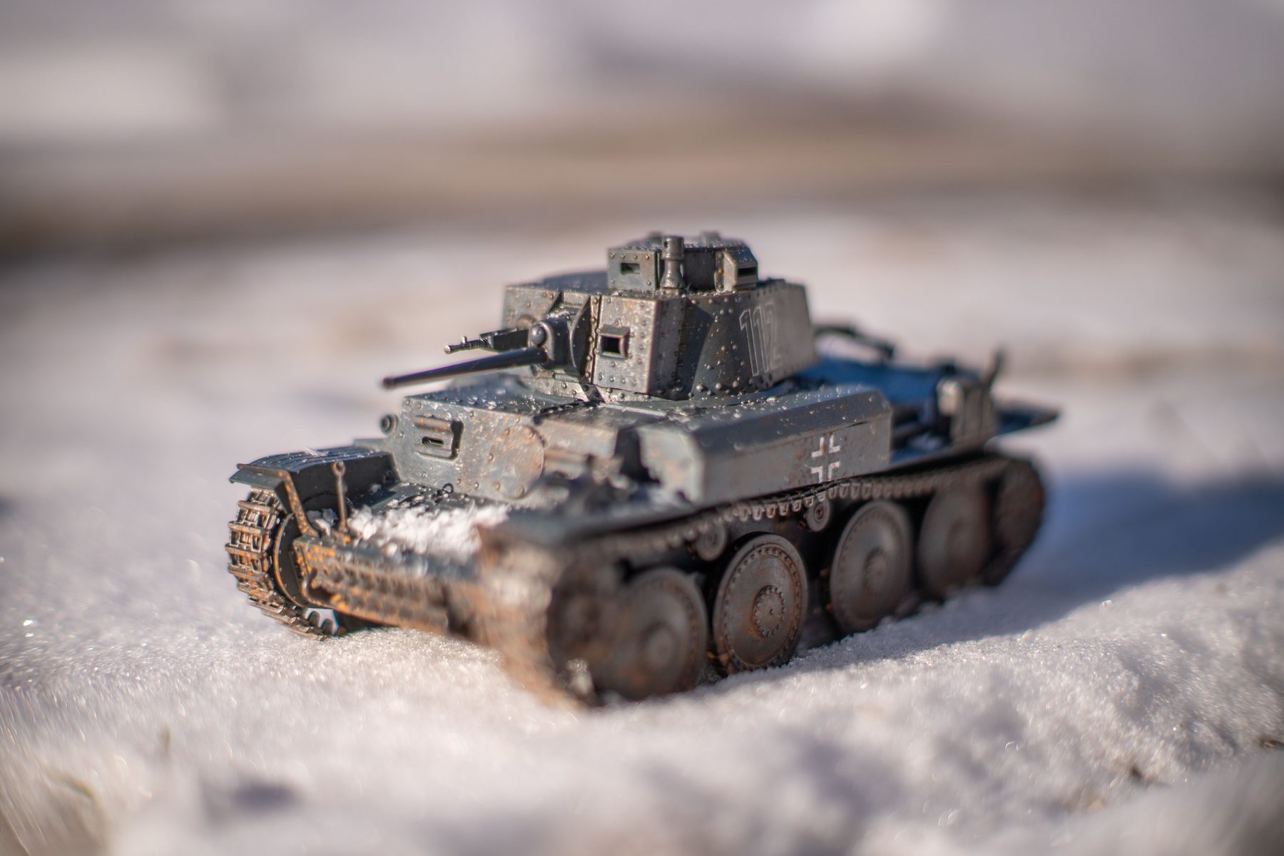
In 1942 the Allies needed a number: how many tanks was Germany building each month? The answer decided how many Shermans had to cross the Atlantic, and it came from spies, prisoner interrogations, aerial photographs of factory roofs, and educated guessing. Those sources agreed on an alarming figure of around 1,400 a month.
They were wrong by a factor of five. A much better number was already sitting in a warehouse, stamped into the gearboxes of wrecked panzers.
Tanks are only the famous case. The method needs nothing military: it works on anything numbered from one upward, in order, wherever you can see a few of the numbers and none of the total. Stand on a corner in a city you do not know, note the licence numbers on the first five taxis that pass, and you can put a figure on how many the city licenses. Statisticians teach it that way often enough that it has a second name, the taxicab problem. The same arithmetic counts the print run of a numbered edition from the three copies you have seen, or the machines a factory has shipped from the plate on the one in front of you, or how many customers a company signed up last month from the ID it put in your receipt. Any sequence somebody kept tidy for their own convenience will answer the question, and the last section of this post comes back to what that means for the tidy sequences around you today. First, the tanks.
The one assumption that does all the work
German factories numbered their parts sequentially: gearboxes, chassis, engines, and, most usefully, the rubber road wheels, whose moulds carried a serial and a date. Sequential numbering means the serials on the tanks that were built form the set \(1, 2, \ldots, N\), where \(N\) is the thing you want to know.
The tanks the Allies captured or destroyed are a sample from that set. If you are willing to treat the sample as if it were drawn at random (and that is the assumption doing all the work here), then the serials you hold tell you something quite precise about the serials you don't.
The intuition: mind the gaps
Say you have recovered four tanks, with serial numbers 82, 214, 507 and 793.
Four numbers cut the line into five stretches: the run up to the first tank, the three runs between tanks, and the run from the last tank up to \(N\). The four you can measure come out at 82, 132, 293 and 286.
Here is the whole idea. If the sample really was random, there is nothing special about the last gap. It is the same kind of gap as the other four, drawn from the same process, so on average it is the same size. Four gaps below the largest serial average \(793/4 \approx 198\), so the fifth should be about 198 as well:
- \(\hat{N}\)
- the estimate of the fleet size. The hat means "reconstructed from the sample", as against \(N\), the true number, which nobody outside the German ministry ever saw.
- \(m\)
- the largest serial you hold. Here 793.
- \(k\)
- how many tanks you captured. Here 4.
- \(\tfrac{m}{k} - 1\)
- one average gap, and the whole trick. Your \(k\) tanks occupy \(k\) of the numbers at or below \(m\), so the stretches between them hold \(m - k\) unseen serials in total, which is \((m-k)/k = m/k - 1\) apiece. Add one more such stretch above \(m\) and you have the top of the run.
That is the entire estimator. It is the minimum-variance unbiased estimate of \(N\), and it fits in one line of code.
Why "the biggest one I've seen" is not the answer
The obvious estimate is \(m\) itself: you have seen tank 793, so at least 793 were built. It is obviously a lower bound, and that is exactly the problem: it is always a lower bound, so it is wrong on average, every time, in the same direction. The size of the error is not a mystery either:
- \(\mathbb{E}[\,\cdot\,]\)
- the expected value: the average of a quantity over every sample you could have drawn, not the value of any one sample.
- \(\mathbb{E}[m]\)
- where the largest serial in a sample lands on average. Always below \(N\), which is the bias.
- \(\frac{k}{k+1}\)
- read the formula as \(N+1\) shrunk by this fraction. The \(k\) serials cut the run into \(k+1\) stretches of equal average length, and \(m\) sits at the top of the last but one, so it lands about \(k/(k+1)\) of the way up: four-fifths of the way at \(k = 4\), twelve-thirteenths at \(k = 12\).
With four tanks in hand you expect to see about four-fifths of the true total. The correction term \(m/k - 1\) is precisely what closes that gap, and the chart below is that sentence drawn: a simulated fleet of exactly 1,000 tanks, sampled over and over, with the average of each estimate plotted against the number of tanks captured.
One captured tank tells you, on average, that the fleet is twice as large as its serial number. Twelve tanks and the raw maximum is still 8% short. The corrected line is flat on the truth throughout. That is what unbiased means, and it is not a coincidence but the reason this estimator is the one you use.
How much can you trust it?
Unbiased on average is a weak promise if any single estimate can be wildly off, so the honest question is how much the estimate moves around. It moves less than you would guess:
- \(\operatorname{Var}(\hat{N})\)
- the variance of the estimate: how far it scatters from one sample to the next. Its square root is the typical error, which is the number worth quoting. At \(N = 1000\) and \(k = 4\) that is about 204 tanks; at \(k = 10\), about 91.
- \(N - k\)
- the serials still unseen. The closer your sample comes to the whole fleet, the less room the estimate has to be wrong, and at \(k = N\) the variance is zero because you are no longer estimating anything.
- \(k(k+2)\)
- the term that pays you for captured tanks. It grows like \(k^2\), so the typical error falls roughly like \(1/k\) rather than the \(1/\sqrt{k}\) you get from averaging measurements.
The \(k^2\) in the denominator is the good news: precision improves roughly in proportion to the number of tanks you capture, not to its square root. Doubling your captures halves your error bar.
A single tank is nearly useless: the 90% range runs from 101 to 1,899. Five tanks brings it to roughly 660–1,190. Ten tanks gets you 816–1,094, an interval you could plan a war around. This is the part that surprises people: the sample sizes that make this work are absurdly small, because each new serial number is not just another observation, it is another constraint on where \(N\) can possibly be.
You do not have to take my word for any of it. Drag the slider and watch both distributions move:
At k = 1 the corrected estimate is a smear across the whole axis: one tank really does tell you almost nothing. By k = 10 it is a narrow pile centred on the dashed line, while the largest serial seen is still visibly short of it and always will be: it has a hard ceiling at the truth, which is another way of saying it is biased.
The simulation is small enough to read in one sitting. In Python:
import random


def estimate_fleet(serials: list[int]) -> float:
    """The estimator: the largest serial, plus one average gap, minus one."""
    m = max(serials)
    return m + m / len(serials) - 1


def sample_serials(N: int, k: int, rng: random.Random) -> list[int]:
    """k distinct serials from 1..N."""
    seen: set[int] = set()
    while len(seen) < min(k, N):
        seen.add(rng.randrange(1, N + 1))
    return list(seen)


def simulate(N: int, k: int, trials: int, seed: int) -> dict[str, float]:
    """Repeat it, and average both estimates."""
    rng = random.Random(seed)
    sum_estimate = sum_max = 0.0
    for _ in range(trials):
        m = max(sample_serials(N, k, rng))
        sum_estimate += m + m / k - 1
        sum_max += m
    return {
        "mean_estimate": sum_estimate / trials,
        "mean_max": sum_max / trials,
}That is the entire experiment. Twenty thousand simulated wars, and the average of the corrected estimate lands on 1,000 whatever value of k you pick, while the average largest-serial-seen lands on k/(k+1) of it, exactly as the algebra above says it must.
What it got right
The statisticians in the Economic Warfare Division did this with real serials from gearboxes, chassis and wheel moulds, cross-checking the three streams against each other. After the war their estimates were compared with the captured production ledgers:¹
| Month | Statistical estimate | Intelligence estimate | German records |
|---|---|---|---|
| June 1940 | 169 | 1,000 | 122 |
| June 1941 | 244 | 1,550 | 271 |
| August 1942 | 327 | 1,550 | 342 |
The conventional intelligence estimates are off by factors of three to eight, and they are off in the direction that costs the most: always too high, always arguing for more caution and more materiel. The serial-number estimates are within a few dozen tanks, from a handful of wrecks and no spies at all.
Where it breaks
The estimator is one line, but the assumption underneath it is load-bearing, and it is worth being explicit about what would break it:
- Non-sequential numbering. The Germans could have defeated this entirely by randomising their serials, or by inserting gaps. They eventually did obfuscate some of it; the wheel moulds, which nobody thought of as intelligence, kept talking longest.
- Non-random sampling. Captured tanks are the ones that fought and lost, which is not the same as a uniform draw from the production line. If newer tanks are concentrated on a front you are not fighting on, your sample skews old and low.
- Multiple factories, multiple lines. Several independent sequences look like one sequence with strange gaps. You have to segment first and estimate each run separately, which is exactly what the Allies did with gearbox marks.
- The number you actually want. \(N\) is total tanks built, and what a general wants is tanks available, which means subtracting everything already destroyed and everything not yet delivered.
None of these are reasons not to do it. They are reasons the answer arrives with an error bar, which is more than the spies were offering.
The general shape of it
Strip the tanks out and the pattern is one you meet constantly: you observe the maximum of a sample and want the maximum of the population. Sequentially numbered anything (order IDs on receipts, invoice numbers, database primary keys leaked in URLs, ticket numbers on a support queue) carries the same information, and the same one-line correction applies.²
It is a good reminder that the sharpest analysis is not always the most sophisticated. Somebody noticed that the enemy had, for perfectly sensible manufacturing reasons, been writing down the answer on every tank they built.